Note: I use the convention that \(\mathbf{a}\) denotes a column vector and \(\mathbf{a}^t\) a row vector, and if \(A\) is a matrix, then \((A)_{ij} = a_{ij}\) denotes the entry in the \(i\)th row and \(j\)th column.
Problem 1
Part 1
Let \(A = (a_{ij})\) and consider \(\mathbf{\epsilon}_{ij}\), the matrix with a \(1\) in the \(i\)th row and \(j\)th column and zeros elsewhere.
Then, for a fixed \((i, j)\), if we write \(A = [\mathbf{a}_1^t, \mathbf{a}_2^t, \cdots, \mathbf{a}_n^t]\) as a block matrix of column vectors, we have \begin{align*} A \mathbf{e}_{ij} = [0, 0, \cdots, \mathbf{a}_i^t, 0, \cdots, 0] \end{align*} as a block matrix where \(\mathbf{a}_i^t\) occurs as the \(j\)th column.
In other words, right-multiplication by \(\mathbf{e}_{ij}\) selects column \(i\) from \(A\), placing it in column \(j\) of a matrix of zeros.
For example, for \((i, j) = (3, 2)\) we have
\begin{align*} A \mathbf{e}_{32} = \left(\begin{matrix}a_{11}&a_{12}&a_{13}\\a_{21}&a_{22}&a_{23}\\a_{21}&a_{22}&a_{33}\end{matrix}\right) \left(\begin{matrix}0&0&0\\0&0&0\\0&1&0\end{matrix}\right) = \left(\begin{matrix}0&a_{13}&0\\0&a_{23}&0\\0&a_{33}&0\end{matrix}\right), \end{align*}
which is a matrix that contains column \(3\) of \(A\) (the \(i\) value) as its \(2\)nd column (the \(j\) value).
On the other hand, left multiplication by \(\mathbf{e}_{ij}\) selects the \(j\)th row of \(A\) and places it the \(i\)th row of a zero matrix, so for example we have
` \begin{align*} \mathbf{e}{32} A = \left(\begin{matrix}0&0&0\0&0&0\0&1&0\end{matrix}\right) \left(\begin{matrix}a{11}&a_{12}&a_{13}\a_{21}&a_{22}&a_{23}\a_{21}&a_{22}&a_{33}\end{matrix}\right)
\left(\begin{matrix}0&0&0\0&0&0\a_{21}&a_{22}&a_{23}\end{matrix}\right) \end{align*} `{=html}
In general, these two products will not be equal, since the first has a nontrivial column and the latter has a nontrivial row. If \(A \in Z(M_n(R))\), these two must be equal, so we can equate corresponding entries to find that
- \(a_{21} = 0\), from comparing entries in row 3, column 1,
- \(a_{23} = 0\), from comparing entries in row 3, column 3
- \(a_{22} = a_{33}\) by comparing entries in row 3, column 2.
Letting the multiplication run over all possibilities for \(\mathbf{e}_{ij}\) yields \(a_{ii} = a_{jj}\) for every pair \(i, j\) and \(a_{ij} = 0\) whenever \(i\neq j\). Setting \(r = a_{ii} = a_{jj}\) for all \(1\leq i,j \leq n\) forces \(A\) to be a matrix of the form
\begin{align*} A = \left(\begin{matrix}r&0&0&\cdots&0\\0&r&0&\cdots&0\\\vdots&\vdots&\vdots&\ddots&\vdots\\0&0&0&\cdots&r\end{matrix}\right) \coloneqq r I_n. \end{align*}
To see that we must have \(r\in Z(R)\), let \(sI_n \in Z(M_n(R))\) be arbitrary, where \(s\) is not assumed to be in \(Z(R)\). Then \((rI_n)(sI_n) = (sI_n)(rI_n)\) by assumption, since these are matrices in the center of \(M_n(R)\). But \(M_n(R)\) is an \(R{\hbox{-}}\)module, and so the scalars \(r,s\) commute with the module elements \(I_n\). This means that we in fact have
\begin{align*}
(r I_n) (s I_n) &= (rs) I_n^2 = (rs)I_n, \\
(s I_n) (r I_n) &= (sr) I_n^2 = (sr)I_n \\
&\implies (rs) I_n = (sr) I_n \\
&\implies (rs -sr) I_n = 0_n,
\end{align*}
the \(n\times n\) zero matrix.
But then by equating (for example) the \(1,1\) entry of the matrix \((rs -sr) I_n\) with the corresponding entry in \(0_n\), we find \(rs - sr = 0_R\), which means \(rs = sr \in R\).
Now since \(s\in R\) was arbitrary, we find that \(r\in Z(R)\) as desired.
Part 2
Define a map
\begin{align*}
\phi: Z(R) &\to Z(M_n(R) \\
r &\mapsto r I_n
.\end{align*}
By part 1, this map is surjective. To see that it is also injective, we can consider \(\ker \phi = \left\{{r \in Z(r) {~\mathrel{\Big\vert}~}r I_n = 0_n}\right\}\), which clearly forces \(r=0_R\). It is also a homomorphism of \(R{\hbox{-}}\)modules, since \(\phi(rx + y) = (rx + y) I_n = r(xI_n) + yI_n\).
Thus by the first isomorphism theorem, we have \(Z(R) \cong Z(M_n(R))\).
Problem 2
Part 1
If \(A,B\) are (skew)-symmetric, then \(A^t = \pm A\) and \(B^t = \pm B\) respectively. But then \begin{align*} (A+B)^t = A^t + B^t = \pm A + \pm B = \pm(A + B), \end{align*}
which shows that \(A+B\) is (skew)-symmetric.
Part 2
\(\implies\): Suppose that whenever \(A,B\) are symmetric then \(AB\) is symmetric as well.
We then have \((AB)^t = AB\) by assumption, and then by calculation we have \((AB^t) = B^t A^t = BA\), so \(AB = BA\).
\(\impliedby\): Suppose that \(AB = BA\) and \(A, B\) are symmetric. We want to show that \(AB\) is also symmetric, so we compute \begin{align*} (AB)^t = B^t A^t = BA = BA. \end{align*} \(\hfill\blacksquare\)
Now let \(B \in M_n(R)\) be arbitrary. We have
- \((BB^t)^t = (B^t)^t B^t = BB^t\), so \(BB^t\) is symmetric,
- \((B + B^t)^t = B^t + (B^t)^t = B^t + B = B + B^t\), so \(B + B^t\) is symmetric,
- \((B - B^t)^t = B^t - B = - (B + B^t)\), so \(B-B^t\) is skew-symmetric
Problem 3
Definition: We say \(A \sim B\) in \(M_n(R)\) \(\iff\) there exists an invertible \(P\) such that \(B=PAP^{-1}\).
-
Reflexive, \(A\sim A\):
Take \(P = I_n\) the identity matrix.
-
Symmetric, \(A\sim B \implies B \sim A\):
\(B = PAP^{-1}\implies BP = PA \implies P^{-1}B P = A\), so we can take \(Q = P^{-1}\) to yield \(A = Q B Q^{-1}\).
-
Transitive, \(A\sim B \& B\sim C \implies A \sim C\):
If \(B = PAP^{-1}, C = QBQ^{-1}\), then \(C = Q(PAP^{-1})Q^{-1}= (QP) A (QP)^{-1}\), so take \(L = QP\) to yield \(C = LAL^{-1}\).
Definition: We say \(A \sim B\) in \(M(n\times n, R)\) \(\iff\) \(B = PAQ\) with \(P \in \operatorname{GL}(n, R), Q \in \operatorname{GL}(m, R)\).
-
Reflexive, \(A\sim A\):
Take \(P = I_{m, n}\) the matrix with \(1\)s on the diagonal and zeros elsewhere, and \(Q = P^t\).
-
Symmetric, \(A\sim B \implies B \sim A\):
\(B = PAQ \implies BQ^{-1}= PA \implies P^{-1}B Q^{-1}= A\), so we can take \(S = P^{-1}, T = Q^{-1}\) to yield \(A = Q B T\).
-
Transitive, \(A\sim B \& B\sim C \implies A \sim C\):
If \(B = PAQ, C = RBS\), then \(C = R(PAQ)S = (RP) A (QS)\), so take \(L = RP, M = QS\) to yield \(C = LAM\).
Problem 4
Lemma: The rank-nullity theorem holds over division rings.
Proof: A linear map \(\phi: D^m \to D^n\) induces a short exact sequence: \begin{align*} 0 \to \ker \phi \to D^m \xrightarrow{\phi} \operatorname{im}\phi \to 0 \end{align*}
But every module over a division ring is free; in particular, \(\operatorname{im}\phi \leq D^n\) is a module over \(D\) and is thus free. So by a lemma in class, since the right-most term is a free module, this sequence splits and we have \begin{align*} D^m \cong \ker \phi \oplus \operatorname{im}\phi \end{align*}
and taking dimensions yields \begin{align*} m = \dim \ker(\phi) + \operatorname{rank}(\phi). \end{align*} \(\hfill\blacksquare\)
- \(A \in M(n\times m, D)\) has a left inverse \(B \iff \operatorname{rank}(A) = m\):
\(\implies\): Suppose toward the contrapositive that \(\operatorname{rank}(A) < m\), so \(A\) has at least one pair of linearly dependent columns. So wlog write \begin{align*} A = [\mathbf{a}_1^t, \mathbf{a}_2^t, \cdots, \mathbf{a}_m^t] \end{align*} in block form with each \(\mathbf{a}_i\) a column vector, and we can assume that \(\mathbf{a}_1, \mathbf{a}_2\) are linearly dependent.
Now suppose such a left inverse \(B\) were to exist. Write it in block form as \begin{align*} B =[\mathbf{b}_1, \mathbf{b}_2, \cdots, \mathbf{b}_n]^t, \end{align*} so each \(\mathbf{b}_i\) is a row of \(B\).
Now if \(BA = I_m\) is to hold, noting that \((BA)_{ij} = {\left\langle {\mathbf{b}_i},~{\mathbf{a}_j} \right\rangle}\), we must have
\begin{align*}
I_{1,1}  &= {\left\langle {\mathbf{b}_1},~{\mathbf{a}_1} \right\rangle} = 1 \\
I_{1, 2} &= {\left\langle {\mathbf{b}_1},~{\mathbf{a}_2} \right\rangle} = 0 \\
I_{1, 3} &= {\left\langle {\mathbf{b}_1},~{\mathbf{a}_3} \right\rangle} = 0 \\
&\vdots \\
I_{2, 1} &= {\left\langle {\mathbf{b}_2},~{\mathbf{a}_1} \right\rangle} = 0 \\
I_{2, 2} &= {\left\langle {\mathbf{b}_2},~{\mathbf{a}_2} \right\rangle} = 1 \\
I_{2, 3} &= {\left\langle {\mathbf{b}_2},~{\mathbf{a}_3} \right\rangle} = 0 \\
&\vdots
.\end{align*}
But the claim is that this can not happen if \(\mathbf{a}_1, \mathbf{a}_2\) are linearly dependent. To see why, note that the linear dependence supplies elements \(d_1, d_2 \neq 0 \in D\) such that \(d_1 \mathbf{a}_1 + d_2 \mathbf{a}_2 = \mathbf{0}\). But then taking inner products against, e.g. \(\mathbf{b}_1\) (that is, applying \({\left\langle {\mathbf{b}_1},~{{-}} \right\rangle}\) to everything in sight), we obtain
\begin{align*}
d_1 \mathbf{a}_1 + d_2 \mathbf{a}_2 = \mathbf{0} \\
\implies {\left\langle {\mathbf{b}_1},~{d_1 \mathbf{a}_1} \right\rangle} + {\left\langle {\mathbf{b}_1},~{d_2 \mathbf{a}_2} \right\rangle} = {\left\langle {\mathbf{b}_1},~{\mathbf{0}} \right\rangle} = 0 \\
\implies d_1 {\left\langle {\mathbf{b}_1},~{\mathbf{a}_1} \right\rangle} + d_2{\left\langle {\mathbf{b}_1},~{\mathbf{a}_2} \right\rangle} = {\left\langle {\mathbf{b}_1},~{\mathbf{0}} \right\rangle} = 0 \\
\implies d_1 {\left\langle {\mathbf{b}_1},~{\mathbf{a}_1} \right\rangle} + d_2{\left\langle {\mathbf{b}_1},~{\mathbf{a}_2} \right\rangle}  = 0 \\
\implies d_1 + d_2{\left\langle {\mathbf{b}_1},~{\mathbf{a}_2} \right\rangle}  = 0 \\
\implies {\left\langle {\mathbf{b}_1},~{\mathbf{a}_2} \right\rangle} = -\frac{d_1}{d_2} \neq 0
,\end{align*}
which contradicts \({\left\langle {\mathbf{b}_1},~{\mathbf{a}_2} \right\rangle} = 0\) as required by the previous equations.
\(\impliedby\): Suppose \(\operatorname{rank}(A) = m\), so \(A\) has \(m\) linearly independent columns – note that this is all of its columns.
Note: since row rank equals column rank, this also says that \(A\) has \(m\) linearly independent rows, so \(n\geq m\).
Viewing \(A\) as a representative of a map \(\phi: D^m \to D^n\), we find that \(\dim \operatorname{im}\phi = m \leq n\). In particular, from the rank nullity theorem, we have \begin{align*} m = \dim \ker \phi + \operatorname{rank}(\phi) = \dim \ker \phi + m \implies \dim \ker \phi = 0. \end{align*} So \(\ker A = \left\{{\mathbf{0}}\right\}\), and \(A\) represents an injective map \(f_A: D^m \to D^n\).
But any injective set map \(f: S_1\to S_2\) has a left-inverse \(g\) such that \(g\circ f = \operatorname{id}_{S_1}\). So \(f_A: D^m \to D^n\) as a set map has a left inverse \(g_B: D^n \to D^m\) satisfying \(g_B\circ f_A = \operatorname{id}_{D^m}\). But then taking the matrix associated to \(g_B\) yields a matrix \(B \in M(m\times n, D)\) such that \(BA = I_m\) as desired. \(\hfill\blacksquare\)
- \(A\) has a right inverse \(B \iff \operatorname{rank}(A) = n\):
\(\implies\): By a similar argument, supposing that \(\operatorname{rank}A < n\) but \(AB = I_n\) for some \(B\), we find that \(A\) has at least two linearly dependent rows this time, say \(\mathbf{a}_1, \mathbf{a}_2\), whereas we obtain a system of equations of the form \({\left\langle {a_i},~{\mathbf{b}_k} \right\rangle} = \delta_{ik}\) where \(\mathbf{b}_i\) are now the columns of \(B\).
In a similar manner, the linear dependence forces, say, \({\left\langle {\mathbf{a}_2},~{\mathbf{b}_1} \right\rangle} \neq 0\), which is a contradiction.
\(\impliedby\): By another similar argument, we find that \(A\) represents a map \(f_A: D^m \to D^n\), and since \(\operatorname{rank}A = \dim \operatorname{im}A = n\), we find that \(A\) represents a surjective map \(f_A\). Surjective set maps have right inverses, so there is some \(g_B: D^n \to D^m\) such that \(f_A \circ g_B = \operatorname{id}_{D^n}\), and when translated to matrices this yields \(AB = I_{n}\). \(\hfill\blacksquare\)
Problem 5
Part 1
\(\impliedby\): Suppose that \(A\mathbf{x} = \mathbf{b}\) has a solution \(\mathbf{x}\).
Write \(A = [\mathbf{a}_1, \mathbf{a}_2, \cdots \mathbf{a}_m]^t\) in block form with each \(\mathbf{a}_i\) a row of \(A\). By definition, a solution to this equation is a \(\mathbf{x} = (x_i)\) such that for each \(i\), we have \({\left\langle {\mathbf{a}_i},~{\mathbf{x}} \right\rangle} = b_i\) (by carrying out the matrix multiplication).
But
\begin{align*}
{\left\langle {\mathbf{a}_i},~{\mathbf{x}} \right\rangle} &= b_i \\
\implies \sum_{j=1}^m a_{ij} x_j &= b_i
,\end{align*}
which says that the collection \(x_1, \cdots, x_n\) solves the equation \begin{align*} a_{i1} x_1 + a_{i2} x_2 + \cdots a_{im} = b_i \end{align*}
for every \(i\), which is exactly the statement that the \(x_i\) simultaneously solve the given system.
\(\implies\): Suppose that the given system has a simultaneous solutions \(x_1, x_2, \cdots, x_n\), and consider the matrix equation \(A\mathbf{x} = \mathbf{b}\).
Letting \(\mathbf{x} = [x_1, x_2, \cdots, x_n]\), we can rewrite \begin{align*} b_i = a_{i1}x_1 + a_{i2} x_2 + \cdots + a_{im} x_m = {\left\langle {\mathbf{a}_i},~{\mathbf{x}} \right\rangle}, \end{align*}
where \(\mathbf{a}_i = [a_{i1}, a_{i2}, \cdots, a_{im}]\).
But then \(\mathbf{a}_i\) is the \(i\)th row of \(A\), and \(A\mathbf{x} = \mathbf{b}\) has a solution iff there is a \(\mathbf{x}\) such that \({\left\langle {\mathbf{a}_i},~{\mathbf{x}} \right\rangle} = b_i\) for all \(i\), which is exactly what we’ve constructed.
Part 2
Noting that applying a row operation to \(A\) is the same as taking the product \(E A\) for some elementary matrix \(E\), we can write \(A_1 = \left( \prod_{i=1}^\ell E_i \right) A\) and \(B_1 = \left( \prod_{i=1}^\ell E_i \right) B\),
thus
\begin{align*}
A \mathbf{x} &= \mathbf{b} \\
\implies E_\ell A \mathbf{x} &= E_\ell \mathbf{b} \\
\implies E_{\ell-1} E_\ell A \mathbf{x} &= E_{\ell-1} E_\ell \mathbf{b} \\
&\vdots \\
\implies E_1 E_2 \cdots E_\ell A \mathbf{x} &= E_1 E_2 \cdots E_\ell A \mathbf{b} \\
\implies A_1 \mathbf{x} &= B_1
\end{align*}
Part 3
- \(AX=B\) has a solution \(\iff \operatorname{rank}(A) = \operatorname{rank}(C)\):
Note that we can only have \(\operatorname{rank}C \geq \operatorname{rank}A\).
\(\implies\):
Suppose that \(AX = B\) has a solution; then \(\mathbf{b}\) is in the column space of \(A\). But this says that \begin{align*} \mathrm{span}(\left\{{\mathbf{a}_i}\right\}) = \mathrm{span}(\left\{{\mathbf{a}_i}\right\} \cup\left\{{\mathbf{b}}\right\}), \end{align*}
where \(\mathbf{a}_i\) are the columns of \(A\). But then taking dimensions on both sides yields \(\operatorname{rank}A = \operatorname{rank}C\), since the rank of the dimension of the column space.
\(\impliedby\):
Suppose \(\operatorname{rank}A = \operatorname{rank}C\); then the \begin{align*} \dim \mathrm{span}(\left\{{\mathbf{a}_i}\right\}) = \dim \mathrm{span}( \left\{{\mathbf{a}_i}\right\} \cup\left\{{\mathbf{b}}\right\} ), \end{align*}
which says that \(\mathbf{b}_i\) is in the column space of \(A\), and thus \(AX=B\) has a solution. \(\hfill\blacksquare\)
- The solution is unique \(\iff \operatorname{rank}(A) = m\).
\(\implies\): To the contrapositive, Suppose \(\operatorname{rank}(A) < m\). Then by rank-nullity, \(\dim \ker A > 0\), so there is a vector \(\mathbf{v} \neq 0\) such that \(A\mathbf{v} = 0\). But noting that \(\mathbf{x} = \mathbf{0}\) is always a solution to \(A\mathbf{x} = \mathbf{0}\), this yields two distinct solutions.
\(\impliedby\):
Suppose that \(\operatorname{rank}(A) = m\). Then by rank-nullity, \(\dim \ker A = 0\), so \(\ker A = \left\{{\mathbf{0}}\right\}\). Now suppose \(\mathbf{v}_1, \mathbf{v}_2\) are potentially distinct solutions to \(A\mathbf{x} = \mathbf{b}\).
Then,
\begin{align*}
A \mathbf{v}_1 &= A \mathbf{v}_2 = \mathbf{b} \\
&\implies A \mathbf{v}_1 - A \mathbf{v}_2 =  \mathbf{b} - \mathbf{b} = \mathbf{0} \\
&\implies A (\mathbf{v}_1 - \mathbf{v}_2) = \mathbf{0} \\
&\implies \mathbf{v}_1 - \mathbf{v}_2 \in \ker A \\
&\implies \mathbf{v}_1 - \mathbf{v}_2 = \mathbf{0} \\
&\implies \mathbf{v}_1 = \mathbf{v}_2
,\end{align*}
which shows that any solution is unique.
Part 4
We want to show that \(A\mathbf{x} = \mathbf{0}\) has a nontrivial solution \(\iff \operatorname{rank}(A) < m\).
\(\implies\): Suppose \(A\mathbf{v} = \mathbf{0}\) for some \(\mathbf{v} \neq 0\). Then \(\dim \ker A \geq 1\), and by rank nullity we must have \(m = \dim \ker A + \operatorname{rank}(A)\). But this immediately forces \(\operatorname{rank}(A) \leq m-1\).
\(\impliedby\): Suppose \(\operatorname{rank}(A) < m\). Then again by rank nullity, this forces \(\dim \ker A \geq 1\), so \(A\) has a nontrivial kernel and thus there is a nontrivial solution to \(A\mathbf{x} = 0\).
Problem 6
Proof following http://sierra.nmsu.edu/morandi/notes/SmithNormalForm.pdf
The goal is to show that any matrix \(A \in M(m\times n, R)\) is equivalent to a matrix \(D\) of the described form, so \(A = PDQ\) for some matrices \(P,Q\). Since \(S\) is in fact the set of Smith Normal Forms for such matrices, it suffices to show that \(SNF(A)\) can be obtained by left and right multiplication by invertible matrices. Moreover, since row operations can be performed by left-multiplication of elementary matrices, and column operations by right-multiplication.
We proceed by induction on \(m+n\).
For the base case \(m + n = 2\), this can only yield a \(1\times 1\) matrix, and the result holds vacuously.
For the inductive step, we will proceed by considering the top-left \(2\times 2\) block, say \(M = \left[ \begin{array}{cc} a & b \\ c & d \end{array}\right]\), and showing it can be reduced to a block of the form \(M' = \left[ \begin{array}{cc} d_1 & 0 \\ 0 & d_2 \end{array}\right]\) where \(d_1 \divides d_2\). Then the sub-matrix obtained by deleting the row and column containing \(d_1\) is a strictly smaller matrix, allowing the inductive hypothesis to be applied.
Moreover, note that if we are able to perform this reduction by a series of left and right multiplications, this will yields \(A_1 = P_1 A Q_1\), and inductively we will have \(A_{r} = (P_r \cdots P_2 P_1) A (Q_1 Q_2 \cdots Q_R)\), so each matrix will remain equivalent at every step.
Note: since \(R\) is a PID, it is also a Euclidean domain, so we can compute greatest common divisors.
We’ll first reduce the top-left entry and eliminate the bottom-left entry.
Let \(d = \gcd(a, c)\), so we can write \(d = sa + tc\) for some \(s, t\in R\). We would like to construct an operation that replaces \(a\) in \(M\) with \(d\).
So let \(\ell_1, \ell_2\) be parameters to be determined; we can then compute
\begin{align*}
P_1 A = \left[\begin{array}{cc} s & t \\ \ell_1 & \ell_2 \end{array}\right]
\left[\begin{array}{cc} a & b \\ c & d \end{array}\right] =
\left[\begin{array}{cc} d & sb + td \\ \ell_1 a + \ell_2 c & \ell_1 b + \ell_1 d \end{array}\right]
,\end{align*}
where we now only have to choose \(\ell_1, \ell_2\) so that \(P_1\) is invertible.
This lets us engineer an inverse matrix
\begin{align*}
P_1^{-1}\coloneqq\left[\begin{array}{cc} \ell_2 & -t \\ -\ell_1 & s \end{array}\right] \\
\implies P_1 P_1^{-1}&=
\left[\begin{array}{cc} s & t \\ \ell_1 & \ell_2 \end{array}\right]
\left[\begin{array}{cc} \ell_2 & -t \\ -\ell_1 & s \end{array}\right] \\
&=
\left[\begin{array}{cc} s\ell_2 - t\ell_1 & -ts + st \\ \ell_1 \ell_2 - \ell_2 \ell_1 & -t\ell_1 + s\ell_2  \end{array}\right]
,\end{align*}
which just says that we need to pick \(\ell_1, \ell_2\) such that \(s\ell_1 - t\ell_2 = 1\), since the off-diagonal entries vanish because \(R\) is commutative.
But this can be done by writing \(a = d k_1\) and \(c = d k_2\), since \(d\) was their gcd, then \begin{align*} d = sa + tc = s dk_1 + t d k_2 \implies 1 = s k_1 + t k_2, \end{align*}
so just choose \(\ell_1 = k_1, \ell_2 = -k_2\) to yield \(P_1 P_1^{-1}= I_2\).
We can observe that in the matrix \(P_1 A\), since \(d\) divides \(a\) and \(c\), \(d\) also divides \(\ell_1a+\ell_2 c\). So write \(k_1 d = \ell_1 a + \ell_2 c\), we can then perform a row operation by left-multiplying:
\begin{align*}
Q_1  P_1 A\coloneqq\left[\begin{array}{cc} 1 & 0 \\ -k & 1 \end{array}\right]
\left[\begin{array}{cc} d & sb + td \\ \ell_1 a + \ell_2 c & \ell_1 b + \ell_1 d \end{array}\right] =
\left[\begin{array}{cc} d & sb + td \\ 0 & -k(sb + td) + \ell_1 b + \ell_1 d \end{array}\right]
.\end{align*}
We now carry out the same process with the top row instead of the first column. This begins by computing \(d_1 = \gcd(d, sb + td)\), where we can immediately note that \(d_1\) divides \(d\).
We then write \begin{align*} d_1 = d s' + (sb + td)t', \end{align*}
then perform column operations (i.e. right-multiplying by some \(R_1\)) to obtain a matrix of the form \begin{align*} Q_1 P_1 A R_1 \coloneqq \left[\begin{array}{cc} d & sb + td \\ 0 & -k(sb + td) + \ell_1 b + \ell_1 d \end{array}\right] \left[\begin{array}{cc} s' & \ell_3 \\ t' & \ell_4 \end{array}\right] = \left[\begin{array}{cc} d_1 & d\ell_3 + (sb + td)\ell_4 \\ ? & ? \end{array}\right] \end{align*}
where again \(\ell_3, \ell_4\) are parameters that can be chosen to make \(R_1\) invertible.
We can again observe that \(d_1\) divides the top-left and (now) the top-right entry, which means we can find a \(k'\) such that
\begin{align*}
Q_1 P_1 A R_1 S_1 \coloneqq
\left[\begin{array}{cc} d_1 &  d\ell_3 + (sb + td)\ell_4 \\ ? & ? \end{array}\right]
\left[\begin{array}{cc} 1 & 0 \\ -k' & 1 \end{array}\right] =
\left[\begin{array}{cc} d_1 & 0 \\ ? & ? \end{array}\right]
,\end{align*}
which puts us back in the original situation.
We can then continue by obtaining a \(d_2\) that divides \(d_1\), doing row operations, and obtaining a matrix of the form \begin{align*} P_2 Q_1P_1 A R_1 S_1 \coloneqq\left[\begin{array}{cc} d_2 & ? \\ 0 & ? \end{array}\right], \end{align*} and so on.
In a PID, “to divide is to contain” for ideals, so this generates a sequence of ideals \begin{align*} (d) \subseteq (d_1) \subseteq (d_2) \subseteq \cdots \end{align*} and since every PID is Noetherian, this increasing chain of ideals eventually stabilizes.
This means that after finitely many steps, we find \(d_{N+1} \coloneqq\gcd(d_N, \cdots) = d_N\),
obtain a matrix \begin{align*} N \coloneqq\left(\prod_i Q_i P_i \right) A \left( \prod_i R_i S_i \right) = \left[\begin{array}{cc} d_N & x \\ y & z \end{array}\right] \end{align*}
where either
- \(x=0\) and \(y\) divides \(d_N\), or
- \(y = 0\) and \(x\) divides \(d_N\).
Without loss of generality, supposing the first case holds, we can write \(d_N = \alpha y\); then
\begin{align*}
E N \coloneqq
\left[\begin{array}{cc} 1 & 0 \\ 1 & -\alpha \end{array}\right]
\left[\begin{array}{cc} d_N & 0 \\ y & z \end{array}\right] =
\left[\begin{array}{cc} d_N & 0 \\ 0 & z \end{array}\right]
,\end{align*}
where \(E\) is again invertible, yielding a diagonal matrix.
Note: in the general case of an \(m\times n\) matrix, this eliminates entries \(1,2\) and \(2,1\). Eliminating the remaining entries in row 1 and column 1 proceed similarly, and never perturb entries that were made zero in a previous step.
Since it is not necessarily the case that \(d_N\) divides \(z\) here, a small additional modification is needed. This is accomplished by a series of row operations, as described here:
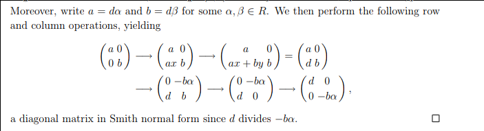 \
\
This yields the desired form in the top-left \(2\times 2\) block, zeroing out the first column and row, so the inductive hypothesis applies to the remaining block. \(\hfill\blacksquare\)